 To start off, what is a customised format? We all understand formatting means the way an item be it a word or a number, is displayed. Bold italic, large or small font size, with a leading ‘£’ for currency or a comma between thousands. We know how to change the formatting. By selecting the item or whole cell or indeed a range of cells and selecting the corresponding tool from Home Tab Ribbon.
Great, nice and easy and effective.
But what do I mean by customised? Well making the item look the way you need it to be easily understood and different to the basic formatting. Not having to spend time in selecting the several available formats, but quickly with one click. Even being able to create a whole new “look”.
Customizing formats
When you select a cell using the right mouse button you see a list and mini toolbar like this. 
In the red ellipse you can see the tool [Format Cells…]
- Select that tool.


This dialog box appears.
At the bottom of the list in the Number tab is the [Custom] section.
Selecting that reveals this dialog box with lots of items already for you to select from as a starting point. 
For instance there is not a tool in the ribbons that allow you to have a cell display the date and time. In this list scroll down to find just that.
You are looking for this. 
But what if you need to display a word as well as a number and need to use that number in a calculation? After all, Excel will ignore cells that are words for a calculation.
Creating your own customised format
In this example, I am going to need the word [Priority] in front of any number I type into that cell.
You are already in the custom section of formatting cells in the number tab. 
- Decide how you would like the number to be formatted, i.e. two decimal points.
For my example, I will select the whole number only.
- Click in the Type area to the left of the [0].
- Type the open [double quotes].
- Type in the word [Priority and a space].
- Type in the closing [double quotes].
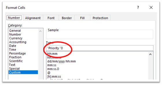
- Its should now read [“Priority “0]
- Select the [OK button]
- If you need this in a range of cells autofill the empty formatted cell to the range you require.
- Type in numbers in that range.
This is what you should see. 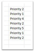
Now you know how to create a custom format, please enjoy yourself and make your spreadsheet more meaningful without not being able to use calculations.


