
Many of us use conditional formatting which changes the colour of a cell where a calculation result sits. This is to easily identify items that meet certain criteria we set. Sometimes you may require to change the entire row of a list not just one cell. To do this, follow these instructions.
Open the list you need to colour.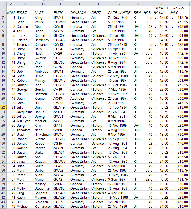
- Select the rows
- Select from the Home tab the Conditional Formatting tool.

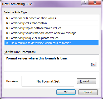
- From the list that drops down Select New Rule…


- From the Select a Rule Type: choose Use a formula to determine which cells to format

- Type the following formula in the dialog box.
=indirect(”E”&ROW())=”Canada”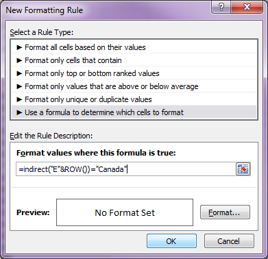
Where E is the column name where your condition lies, and Canada is your condition.
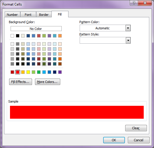
- Now select the Format… button
 in this dialog box to choose the colour you require.
On selecting OK twice your spreadsheet immediately is formatted. Here is what it can look like.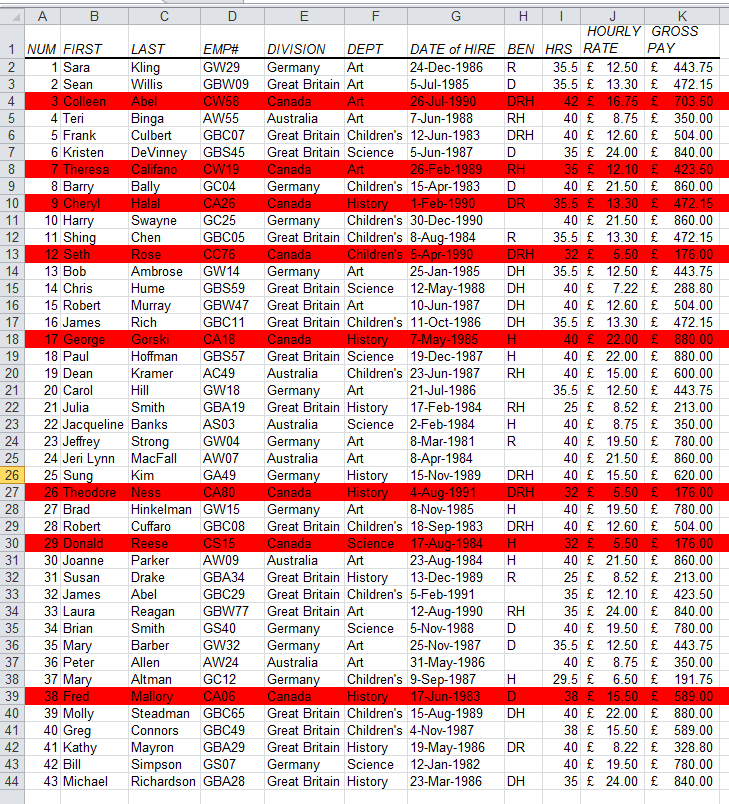
The beauty of having conditional Formatting Rules is that you can revisit them and edit them at will or add to the list of conditions.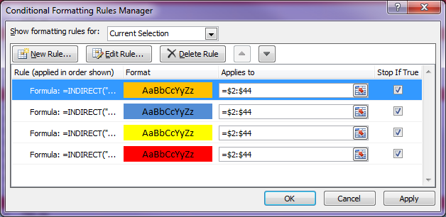
Resulting in 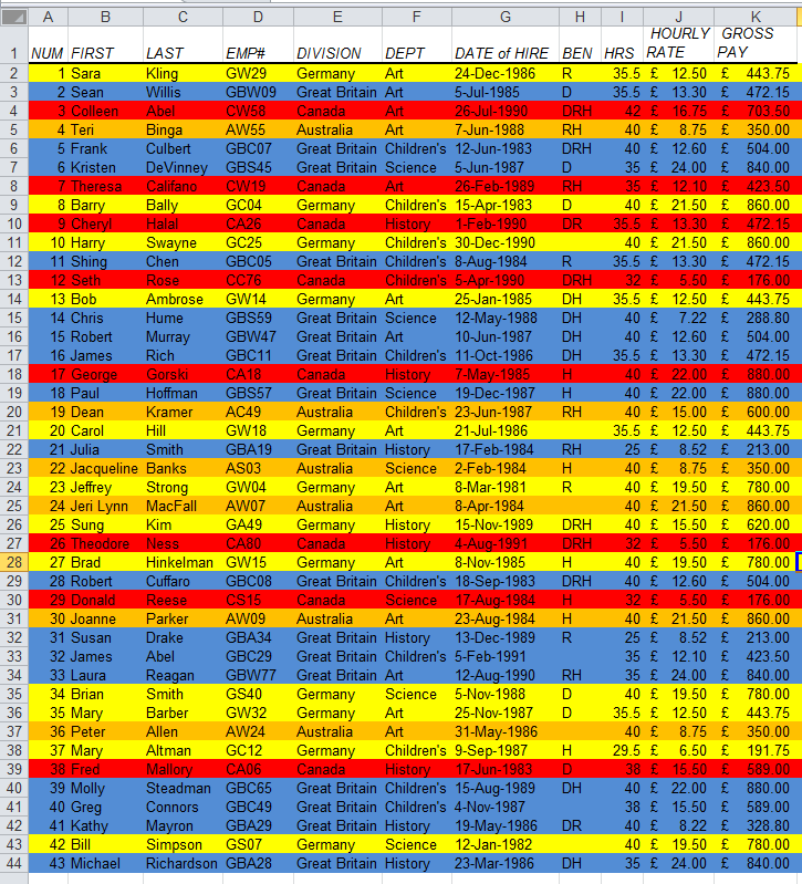
You can also sort by colour of cells.


