 There are many different situations where we need to colour cells in Excel to help us understand the data more quickly. To be able to see correlations between items more easily. When I teach, I often find people doing things the very long way round which not only takes time but also introduces potential mistakes.
I am going to investigate the ability to have a particular list of items which are coloured to change the background colour of another cell. Here is the scenario.
I need to see quickly who on my team is working on which projects for which client. Therefore, colour coding helps enormously. I have in the past shown you how to use Conditional Formatting, Absolute referencing, nesting functions and data validation rules both values and lists. I suggest you familiarize yourself with these if you don’t already use these features. Here I am going to use all four features together.
How to set up your data sheet
My spreadsheet has a list of clients my team are working on for different clients. I am selecting the names of my team to be the control for the colour coding.
- On a new sheet, not in the one your data and calculations are on, type the list of possibilities that you will need to select from when you input new data on the data sheet.
My list is names of the team.

I have chosen to colour the background here of each item for future reference. (This will not translate when I use the data validation rule in a cell.)
- Name this sheet as “Lists”, you may be creating a few more for various other reasons later in the calculation stages.
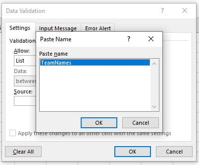
- Select the list and name it. For example – “TeamNames”.
- In the sheet where your data is, where you need to colour cells. Create the Validation rule in the cell where you require a name of one of your team. Here you will select List from the Allow:
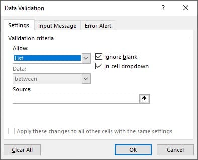
- The list is the one you have just created and named “TeamNames”.
My list of team members and clients looks like this.

My team members are in column I but clients surnames are in column C. this is the second sheet Sheet 1 is named Lists where my team members are found.
- In this sheet of clients, select the the first cell (C2) where you need to colour the background in the same colour as the team members name, working with that client.
- Select Conditional Formatting from the Data tab.
- Select New Rule from the list.
- Select the “Use a formula to determine which cells to format”.
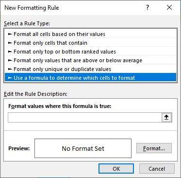
- Type the following formula into the next box “Format values where this formula is true”.
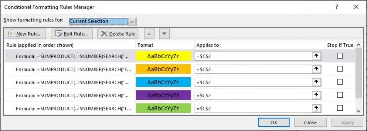
=SUMPRODUCT(- -ISNUMBER(SEARCH(“fred”,$B2)))>0
Note:
- type two hyphens before the “isnumber” with no space between.
- my $I2 refers to the cell where the name of my staff sits.
- make sure that you have the same amount of opening brackets as ending brackets.
- Select the Format… button to select the correct colour for the background.
- Select OK button.
You will need to do this for each team member.
Once you have created all the rules for each member, review the list to make sure you have all the names covered.
Select the Manage rules from the conditional formatting tool list.
- Select the OK button to finish.
- Use the Format Painter tool to paint the formatting background colours to the rest of the column of clients.
How to use the conditional formatting
- Select the first cell where you can fill in by selecting from the dropdown list a name of your team member. (Having used the data validation rule.)
- When you select that name the cell you have created the conditional formatting will automatically colour that cell accordingly.

I have partially filled the column with my team members names but the result looks like this.

Note: that the names are not case sensitive. In the cell A1 I have typed Dick whilst in A6 I have typed dick but I still have the result in column E with the correct colour.
Note also that this conditional formatting formula does not require the data validation but I feel it is always better to select the name rather than possibly type the wrong letters and get the wrong result.


