 There are lots of wonderful features in Excel now to make reporting on data easy and fun. But sometimes all you really need is a simple function. There are hundreds of functions in Excel and I have shown you a few that are almost absolutely necessary to know when working in Excel.
Here is a list of those you can find on Enterprise Times:
- The Sum Function
- Functions in Excel
- The If Function
- Today Function
- The Count function
- More on Count
- The PMT Function
- The VLookup Function
- Using Range in the VLookup Function
There are three parts to the IF function; the condition, what to do if that condition is met, and what to do if that condition is not met. Using the SUMIFS function you can use several conditions at the same time. Let’s see how this is put together.
Here is a simple spreadsheet to work on. 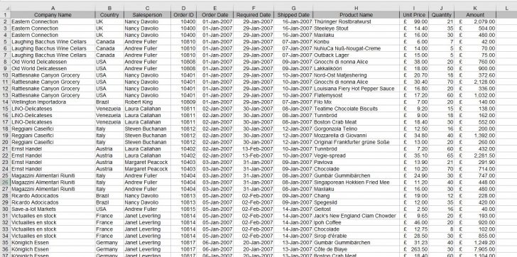 We need to find what the total amount comes to for a particular company and a particular sales person. Therefore, we only sum up the amounts if both criteria are met.
The SUMIFS function looks like this. (Known as the syntax)
=SUMIFS (sum_range, range1, criteria1, [range2], [criteria2], …)
The syntax explained:
sum_range – The range to be summed.
range1 – The first range to evaluate.
criteria1 – The criteria to use on range1.
range2 – The second range to evaluate.
criteria2 – The criteria to use on range2.
You can use up to 127 different criteria.
By default, the function only gives you a single result. If you want to use the function against the table above and get a list of how much each salesperson had earned per company, you would want to build a separate table or store the results in a separate sheet.
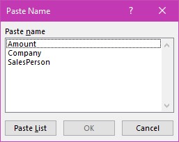
It is good practice to name your ranges for the criteria. It is easier than remembering absolute referencing and makes using the function simpler. In my example I have created three names ranges, one for each of the key areas. It is important to make sure that each range is identical in length.
Here is the Name Manager dialog box to show you what I’ve done. 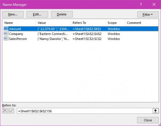
Here is the table for our results. 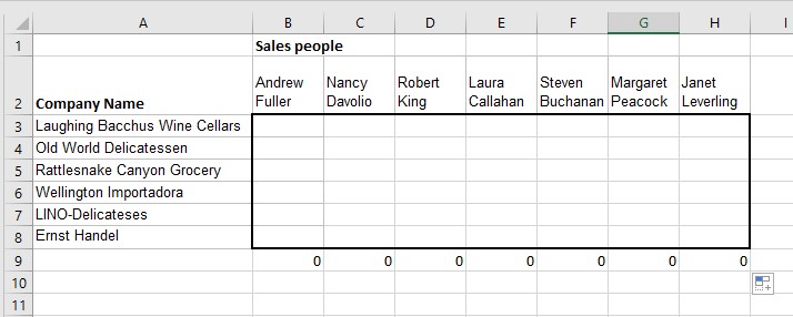 I have placed the names of companies I’m interested in, in column A and sales people in row 2. The SUMIFS function will be in the boxed area B3:H8
In cell B3 place the SUMIFS function using the Insert Function Tool. 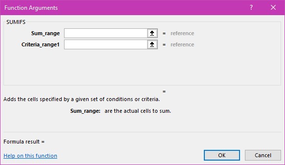
- Click in the Sum_Range box, press F3 to display range names, select “Amount” and click OK

- Click in the Criteria_range1 box, press F3, select “Company” and click OK.
- This will create a third line “Criteria” (see dialog box below)
- Click in the Criteria box and select the cell “A3” which holds the first company name. Make the column an absolute reference and then press OK.
- Click in the Criteria_range2 box, press F3, select “SalesPerson” and click OK.
- Click in the Criteria2 box and select cell B2. Make the Row an absolute reference and press OK.
Here is the finished dialog box. 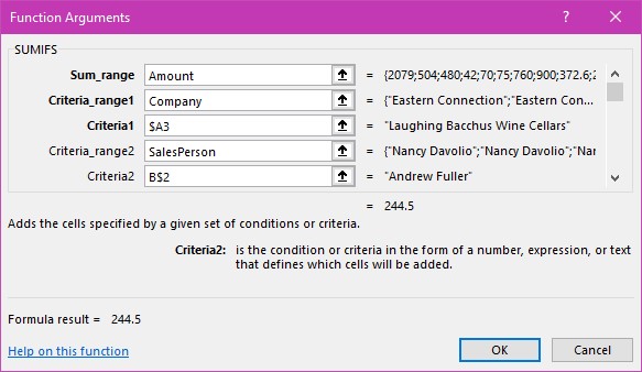
- Autofill down and across the table.
Here is the result. 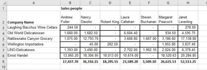
As soon as you change the criteria, for example, one of the company names. The table updates the results automatically.
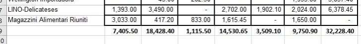
You can insert additional rows into your existing table as you add new company names to your data and new columns as you add sales people.


