
Naming cells or ranges of cells can be a very useful technique in Excel. You might use it to its full potential or just to be able to quickly locate a special area in your workbook. I shall start with this.
You may have several sheets in your workbook and find it cumbersome to locate special areas from which you need to find answers. Using “naming” allows you to quickly go to that area wherever it may be in your 255 sheets, not only that but it is selected for you when you go there, no matter how large it may be.
- Select the cell or cells you wish to name.
- From the Formula Tab
 in the Define Names section Select Define Name Tool
 in my example workbook I have 255 sheets and need to refer frequently to sheet no 251 cell reference M63:M73. By selecting this range, which starts with a word, and selecting the Define Names Tool my dialog box is filled with the correct information.
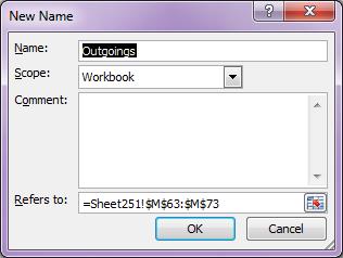
Name: Takes the first cell in the range or touching the range selected. You can replace this name if you wish.
Scope: is the where you wish to be able to use this named range i.e. only in one sheet or for the whole workbook.
NB– Named ranges can only be used in the same workbook.
Comment: You can type some information that will help you understand why you named this range and how you use this name in your workbook, it will still work if you don’t fill this in.
Refers to: This is the location of the data, the sheet name followed by the cell reference with Absolute Referencing in place.
- Select OK
A quicker way
A much quicker way to create a name is to select the area you wish to name.
- Select the Name box which highlights the cell reference.
- Type in the name you wish to apply to this area. You must not use spaces or special characters only alphabet and numbers and the underscore.
How to use named cells or ranges
To use a name just to get to the named range again from anywhere in the workbook go to the Name box which is located just above Column A on the left of your screen.
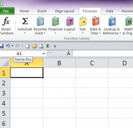
- Select the drop down arrow, this reveals the list of named areas you have created in your entire workbook.
- Click on the one you need and you are whisked off to that place.
You can name several areas at the same time if need be.
- Select the cells you wish to sum together with their respective titles.
- Select Create from Selection Tool from the Formula Tab.

- Select OK as the dialog box is correctly selecting the titles for you to name each separate column by the title at the top of each column.
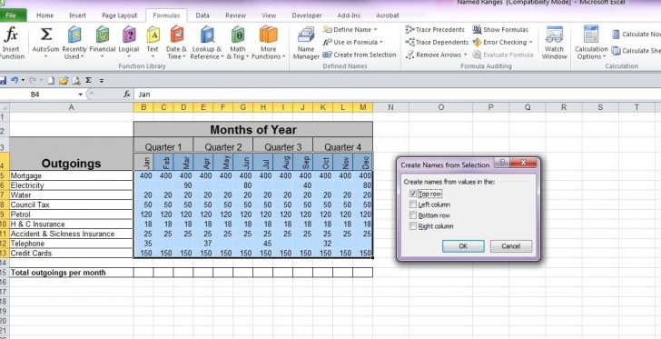
The result is each column of data from row 5 through to 13 now is named Jan through to Dec accordingly.
Using Named ranges within a formula
Its great being able to get around a workbook quickly but it’s even better to be able to understand what a formula is doing for you. What I mean is you can change a what could look like a complicated formula into a sentence you can understand. I shall start by creating a simple formula with range name within it.
You have a list of items that you need to add up and these are displayed in months. If you select the area you wish to calculate i.e. B5:B13 and name it. A sensible name would be Jan. the Formula would read =Sum(JAN). this is almost a sentence “Sum up the Jan figures”
Therefore
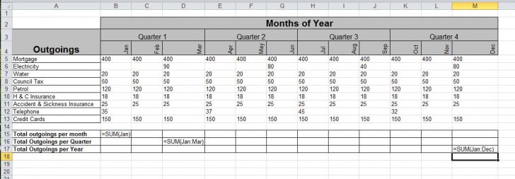
in B15 you would have =SUM(JAN)
in C15 =SUM(FEB)
and so on.
You may wish to sum up just the quarters.
The formula would read; =SUM(JAN:MAR)
For the year the formula would read; =SUM(JAN:DEC)
N.B. You cannot autofill this kind of formula as the names have Absolute Referencing.


