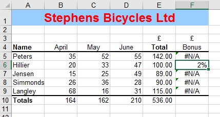
In my last tip, Using Vlookup in ExceI, I explained how to create a Vlookup function. I only showed you how to use the first three lines of this function and missed out the last line which is the Range lookup. This part is used when you wish to find an exact match in your list to the item in your spreadsheet.
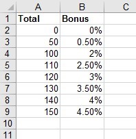
I explained that when you create your lookup list it starts at the smallest value and grows down the sheet in increments of your choice but in order. These are placed in the first column. The second column holds the values that are needed.
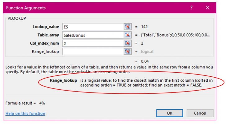
When you use the vlookup function and leave the fourth line blank you are in fact saying that you are looking for the nearest match to the item in your spreadsheet.
As the screen suggests you can type the word TRUE or leave the line blank.
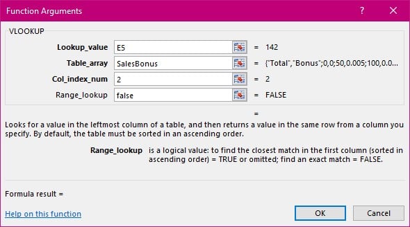
If on the other hand you are looking for an exact match only, you need to type the work FALSE. This is not at all intuitive as the word false conjures up the thought of getting what you are not looking for.
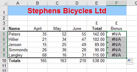
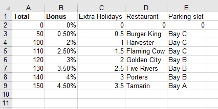
My example has the first column starting at 0 and jumping to 50 then 100 then 110 etc. it does not increment by 1 therefore not all numbers are found here in this first column. Therefore, if you should look for an exact match to a number that does not exist in the list you will have an error message returned.
If you have the number in the spreadsheet that exists in the list, then you will get an answer.
It is therefore very important to create a list that is comprehensive for your needs. This may take some time to create and have the second column hold many repetitions but in the end, well worth the time and effort.
Lookup lists can also be used several times over. What I mean by this is you may wish to return a different answer dependent upon the first columns items. i.e. dependent upon the total sales depends how many days holiday the sales person will receive. Or, which restaurant voucher they will receive. Or, maybe even which parking space they may use for the week. The variants can all be placed in the same lookup list.
Your function now can use any of the 4 columns, or as many as you need, to retrieve the answer you require.
Here is an example of the lookup list.
The answer to the bonus is in column 2 the answer to the holidays is in column 3 and so forth. Please do not forget to create a new range name as this lookup list is bigger and to be used in different calculations therefore the name should reflect this. I suggest something like ‘SalesExtras’.
Therefore, the formula would read something like this:
Now you know how it’s done go and enjoy this lovely function.

