 When you create a spreadsheet the data you type into the cells sometimes does not fit well in the predefined by Microsoft column widths or row heights. You well know that if the data in one cell is too long for the column once you type data in the cell to the right some of the data in the left column disappears from view. Similarly, if you wrap text so that it will not flow into the next column the row height will expand to suit this. But sometimes it won’t be what you need.
Here is an image of the default size of cells in Excel. 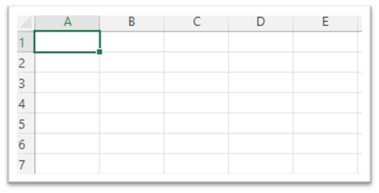
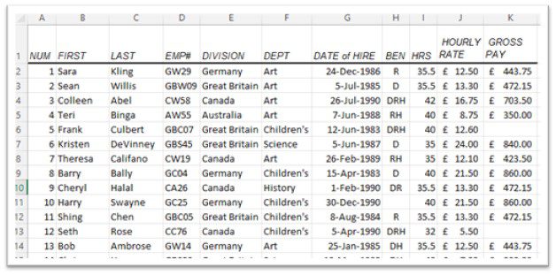
Here is an example of some data not fitting. 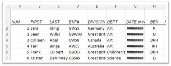
The first thing that jumps out is the column headed [DATE of H] that has hashes in. This is because Excel cannot display a number in full and so gives you warning. It is too easy to misunderstand 100 instead of 1000000 if all you can see is 100.
The next thing is that in the [DIVISION column], some entries are not complete. This is again because Excel cannot display the item in full because of the restriction of the width of column.
Here is an example of text forced to wrap the text down the cell. 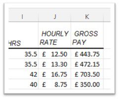
This display allows the numbers to be nearer to each other.
Two ways to change
Column width
1st way
- Select a cell in the column you wish to enlarge or shrink.
- Select Format tool in the Home tab ribbon.

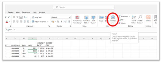
The tool tip appears as your mouse hovers over this tool to explain what the tool does. 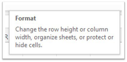
- Click on the dropdown arrow.
This list appears. 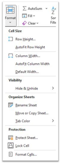
- Select Column Width…
This presents to you. 
The 8.43 is a measurement in Characters. This is dependant upon the typeface you are using. You can type in the exact measure you require. This could be a lot of trial and error to get the width right for the whole column though.
- Select the [OK Button] to change the width of the entire column.
- You can select [AutoFit width column] from the list to choose the best size for you.
- You can also set a default for the whole sheet but selecting [Default Width…]
2nd Way
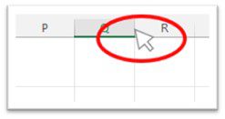
Move your mouse to see an arrow whose tip lies just on the line between two columns. This should be in the header row of columns, to the right of the column you wish to change.
 With the left mouse button, click, hold and drag to the width you require.
 With the left mouse button, click, hold and drag to the width you require.
If you require the best fit, use the double-click and Excel will autofit the column width for you.
Row height
In the same way as above for columns, use the menu for exact or best fit or to change the default of the row height.
There also the ability to use Wrap Text to enlarge the height of a row and see all your text within a cell on multiple lines.
Use the mouse in the header row names below the row you wish to change and click and hold and drag to the size you require or double-click for best fit.
Here is the data sheet with all the columns and rows to specific sizes to show off the data best.
In the next tip I shall show you how to change width or heights to selected columns and rows.


