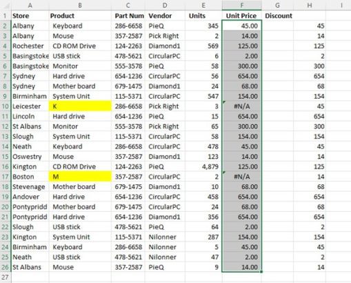
 In my previous tip, I talked about the formula VLookup and its quirky problems. At the end of the tip I showed you a result that gave me #N/A in the cell. That could be fine for some of the time but maybe words would be better to show in a report rather than #N/A.
#N/A means that the information is not available. So let us replace that with a more meaningful and helpful result. Such as the words “No Price Found”.
How to extend a formula.
We used the following formula in the example seen above.
=VLOOKUP(B2,UnitPrice,2,FALSE)
The function we used was “VLookup”
The Lookup value was cell B2
The table array was “UnitPrice”
The column index was 2
And the Range Lookup was False, meaning that we only wanted exact matches not a close match.
We are going to extend this and to accommodate our new need.
How to extend a formula
In this case, we need to add a function in front of the function that has been used.
- Select the cell that holds the first formula F2
- In the formula bar, click at the start of the formula
- Type in the function IFNA with an open bracket but no space between that and the function already there (VLookup)
- Use the [End Key] on your keyboard to quickly move the cursor to the very end of the formula
- Type in a coma [,]
- Type in leading double quotes [“]
- Type in the words you wish to have displayed i.e. [No Price Found]
- Type in the closing double quotes [“]
- Type in the final closing bracket [)]. You should always have equal amounts of opening and closing brackets in a formula
- Press the [Enter Key] on your keyboard
Your formula should look like this. 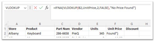
If you should have gone wrong don’t forget that you have the wonderful magic tool of Undo (CTL+Z), 
or if you are still in the formula bar just select the red cross at the start of the formula bar, and you have back what was there before. Just the first formula. 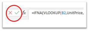
Having pressed the Enter Key on your keyboard you have accepted your changes to the formula and the result should be showing in the first cell F2.
- Autofill this down the page to reveal the new answers.

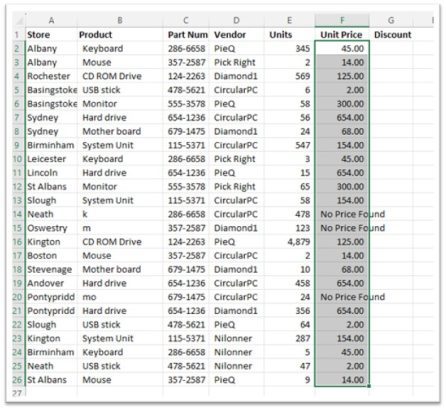
So now you know how to create a more meaningful and user-friendly report in Excel.


