
You have I hope read my two previous tips on how to filter a list in Excel and then how to sort that list. Well there is still more to know about the filtering function. I am sure that there are many of you that filter your lists and think that’s it and put up with the fact that you may need a subtotal of your items but did not know that there is something you can do within your filtered list. This is called Subtotalling. I know, obvious but not quite. You don’t use the subtotalling tool from the Ribbon but the Subtotalling function from the Insert Function list.
Here is a list that has already been filtered at least once. It is very important to know that you have filtered the list at least once otherwise this will not work.
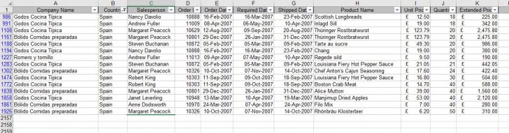
As you can see the list only has the Spanish entries.
Select the cell directly under the last entry of the Extended price column.
Select the AutoSum tool on the Home Tab. ![]()
The formula you get is a little different from the normal. 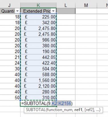
Instead of the usual “=SUM(………” the function Subtotal is used. This is because you have hidden rows and you only want the sum of the visible rows of data. There is a number 9 at the start of the formula inside the brackets. This is the code to sum the range that is following it. There is a list of all the codes for Subtotals Functions found in the Help file in Excel.
If you were to start typing your formula you would get the list like this. 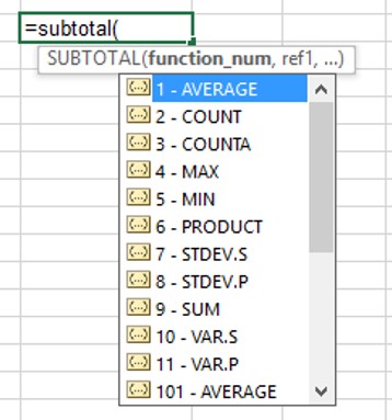
N.B. NEVER try to subtotal a column before you have performed at least one filter action. As you will get the sum of the whole database not just what is on show when you create the filter.


