
I see loads of adverts for all sorts of loans that look so inviting. But wouldn’t you like to see what will be the amount you have to pay back if the rate of interest changes. One such way is to create a Data table in Excel. Using the PMT function to do the calculations.
So what is a data table? Well its basically a cross referencing block of calculated cells that you can use to see what the result is if you have either one or two variables in your formula. This could be very helpful to be able to check if you can afford the loan should the interest rate increase.
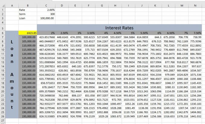
Here is the final result we will work to.
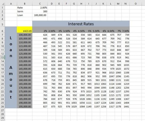
As you can see it is quite a comprehensive set of data.
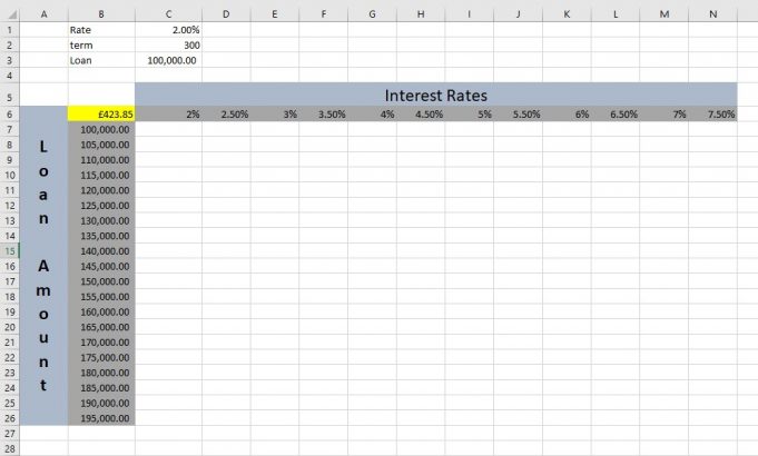
- Type in the cells B1:C3 what you see here.
This is the basis of your PMT function, where the rate is in APR and the length of term is in months.
- Type the PMT function with its arguments or use the PMT function Wizard in the cell B6. The formula should read. =PMT(C1/12,C2,-C3,1).
The result gives you a monthly repayment figure based on a fixed rate, a fixed term and a fixed amount. If you change the entries this will change the repayment figure but it takes time to do so individually. Planning takes longer and becomes frustrating having to change the entries and possibly just remembering the results. If you have a data table the results of every possibility are there to view at any time. And even easier to change the entries.
- Type ‘Interest Rates’ in the cell C5 and centre across the area C5:N5.
- In the cells C6:N6 type in the interest amounts you believe you will need. It might be a good idea to have small increments such as a half a percent.
- In the cell A6 type in ‘Loan Amount’. Then merge and centre the cells A6:A26.
- In the cells B7:B26 Type in the amounts for a loan. Again with small increments.
- Format as required.
Your spreadsheet should look like this.
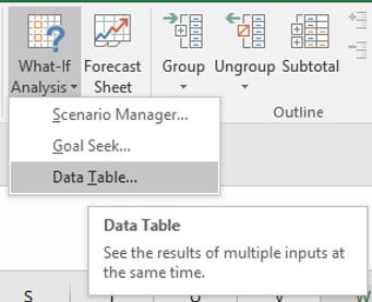
- Now select the area B6:N26. This includes the different amounts and the rates of interest as well as the PMT formula.
- From the Data Tab.

- Select the What If Analysis Tool.

- From the list that displays. Select Data Table at the bottom.
You are presented with a question.
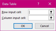
- For the Row input cell select the interest rate in cell C1.
- For the Column input cell select the loan amount you want in cell C3.
- Select OK.
The result looks like this.
You might like to format the numbers to show only whole numbers.
Now change the interest rate in cell C1 and the loan amount in C3 and even the term length in C2 and see what happens to your Data Table results. You will notice that if you change in cells C1 or C3 the Data Table does not change. Only the cell B6 with the PMT formula in will show a different result. If on the other hand you increase or decrease the length of term in cell C2 the Data Table will change.
Hope this tip will come in handy for you.
You could if you like format the results even further like this.
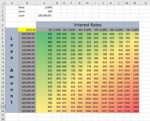
Here I have used the Conditional Formatting Tool and selected the Colour Scales where red is a high number and green is a low number. this makes your choice even easier.
Question: is there more than one cell with the same figure in?


