
Whenever I train Excel and Pivot tables are on the menu I get a varied response. Either people are terrified of them or they just don’t understand how to use them or they just can’t wait to learn about them more. Me – I love them. You may have used Excel for a number of years and possibly used the filtering, sorting and subtotalling with a bit of subtotalling in a filtered list abilities in Excel for your large “database” type of sheet. You’re quite happy with all of this and don’t feel you need anything else. Well keep reading and find out how to create a simple Pivot Table and how it can change your life for the better.
Firstly, we need to look at the data you are going to be working with. Has it been created in Excel or in a database such as Access or some other product and imported. You need to take a good while getting to know your data sheet as lots of pitfalls could stump you. For example, recently I had the pleasure of helping a delegate untangle why his pivot table just won’t run. The reason we found was that he had imported the data from another application that made that data look great and everything in the right place BUT unfortunately it created many merged cells and all the dates came across as text not dates. This made creating a Pivot Table impossible. It was not easy to see the faults and that is why I say take time to familiarise yourself with the data and make sure all is well. Simply put, make it “Clean”.
Here is an example (all be it tiny) of a database type of sheet. 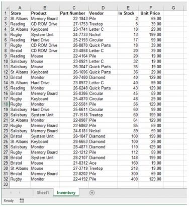
You may need to know which store has a product and how many in stock.
How to create a Pivot Table
Make sure that you are selecting one cell inside the data you have.
From the Insert Tab select the first Icon which is the Pivot Table.

This will lead you to this dialog box.
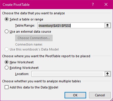
The default is to select all the cells adjoining the one you started with as the data to be worked with on the sheet you are in. Here you can see that the sheet is called Inventory. The exclamation mark is necessary to differentiate the name of the sheet from a name of a range in a sheet. The range that is being used here is A1:F32. Read my tip on Understanding Referencing to understand the dollar signs in the references. These are called Absolute References. By the way don’t forget to include the titles at the top of each column as these are used in your Pivot Table. You may like to name your range of data. See my tip on naming ranges. The area I would choose here and name would be $A:$F.
It is always a good idea to check that the table you will be working from holds all the data that you need and if not, you need to redirect the selection to the correct area.
Today we are not investigating an external data source.
The second part is to decide where you wish your resulting Pivot Table to exist. I suggest that this is always on a separate sheet on its own as when you make amendments it may grow exponentially, so you need a lot of space.
Select the OK button.
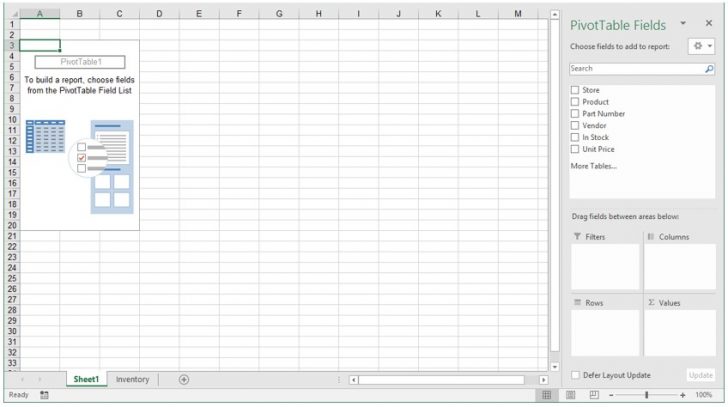
Immediately you can see that a new sheet has been created for you that is empty but for a small blue design in the top left corner. What you may miss the first time is that there is a new window to the right. This shows all the headings found in your data sheet. These are called “Fields”. Underneath the fields is found four areas where we will place the items we are interested in from the field list.
N.B. Give this new sheet a name as you may lose sight of it later on. Stock Pivot Table is a good name. You might wish to create another pivot table with different choices so name your result sheet accordingly.
Click on the fields you require. I suggest for today we select Product, Store and In Stock.
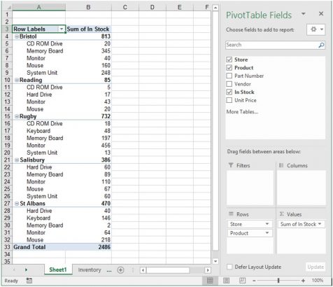
This populates the sheet resulting in your pivot report!
Hey that was a bit quick! Yes, it is that easy.
We now need to make this report easier to read.
Look to the right and notice that the Store and Product fields have both been placed in the Rows area and that the Stock in the Values area and defaulting to “Sum of”.
Drag the Store or the Product to the Columns area.
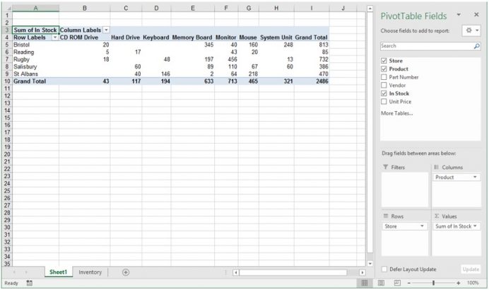
This changes the whole feel of the resulting report.
Swap these fields over and see if this looks better.
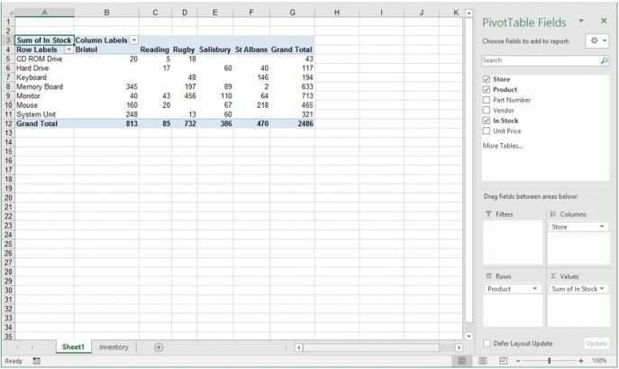
You could argue that they are both just as valid as each other. But bear this in mind as you create your own pivot tables and “play” with the position of your fields to get exactly what you require.
So, there you have your first Pivot Table successfully created and looking great.
Watch out for the next part on Pivot Tables.


