
When I teach Excel to my delegates, there are many who at first think they do not need formulas in their spreadsheets as all they do is sort lists. They don’t realise the potential that formulas can give them. When they do, the If function and the VLOOKUP are most useful. I covered creating and using the IF function in an earlier article. Using the IF Function in Excel. I then went on to explain Using a nested IF Function in Excel. For me the VLOOKUP function goes hand in hand with the IF function.
Firstly, for a lookup function to work you need a list that gives all the possible answers you may need. In the similar way that you create a condition in an IF function you are creating many conditions in the lookup function list.
VLOOKUP is used when a list is created vertically down the sheet.
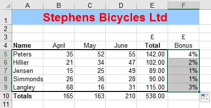
Here is the scenario: You are presented with a sheet of your sales people’s sales figures. You are wanting to give the successful ones a bonus. This will spur on the less successful ones s well.
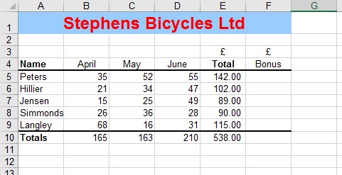
My example is a very small spreadsheet and you probably have tens of sales people. You are not going to go down the list and manually type in the bonus percentage or calculation, dependent upon their total income for the quarter.
- On a separate sheet create a lookup list.
In the first column, the heading will be Total as that is what you will be testing against.
The second column will have Bonus as a heading.
In the Total column, you need to start at the very smallest total your staff could possibly attain. Then grow down the sheet in order. 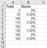
- Now name this area. Refer to my Tip on How to name cells or ranges in Excel .
The name you choose should be a meaningful one that cannot be mistaken for another item. But keep the name as short as possible and don’t forget you cannot have spaces in the name.
- Select the first cell where you need to show the amount of bonus for the first sales person.
- Select the fx button on the formula bar or in the formula tab
- Search for VLOOKUP.
- Select it and you will be presented with this dialog box.

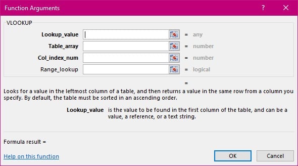
- In the first line of this box select the cell (E5) for the first salespersons total. This is your test.
- Click in the next line in the box for the Table array. This is the name of the list you have made previously. You must use the exact name you created for your list otherwise this formula will not work. Miss typing will lead to errors. You can use the F3 Key from your function keys on your keyboard to display all the named ranges located in your workbook.
- Select the correct one.
- Click in the third line in this box for the col_index _num this is asking you from which column in your vertical list you require the answer from. In our case, it is from the second column, so type in “2”.
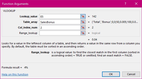
For this scenario, we do not need to use the fourth line. Range_lookup as we are looking for anything that is near to the total in column E. i.e. anyone who gets a total of between 0 and 49 will receive a bonus of 0% anyone who gets a total of between 50 and 99 will receive a bonus of 0.5% and so on. As you can see you have many more possible answers as your spreadsheet has nearly 1.5 million rows so your increments in the first column of your list could be quite small.
Naming ranges makes things so much easier to understand in a few months’ time when you revisit this formula.
- Fill this formula down the column to get all the results.
Check the results are correct. They will be but it’s always a good idea to check anyway.
In my next tip I will explain the Range lookup part of this function as well as having more than two columns in your list.


